.Modelica.Fluid.Utilities.regFun3

Information

Approximates a function in a region between x0 and x1 such that

• The overall function is continuous with a continuous first derivative everywhere.
• The function is co-monotone with the given data points.

In this region, a continuation is constructed from the given points (x0, y0), (x1, y1) and the respective derivatives. For this purpose, a single polynomial of third order or two cubic polynomials with a linear section in between are used [Gasparo and Morandi, 1991]. This algorithm was extended with two additional conditions to avoid saddle points with zero/infinite derivative that lead to integrator step size reduction to zero.

This function was developed for pressure loss correlations properly addressing the static head on top of the established requirements for monotonicity and smoothness. In this case, the present function allows to implement the exact solution in the limit of x1-x0 -> 0 or y1-y0 -> 0.

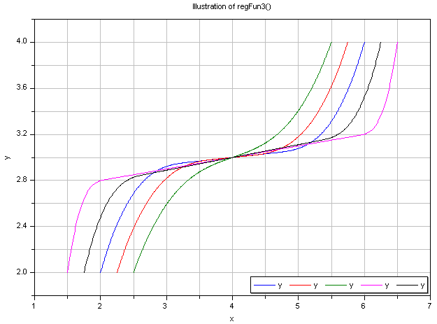
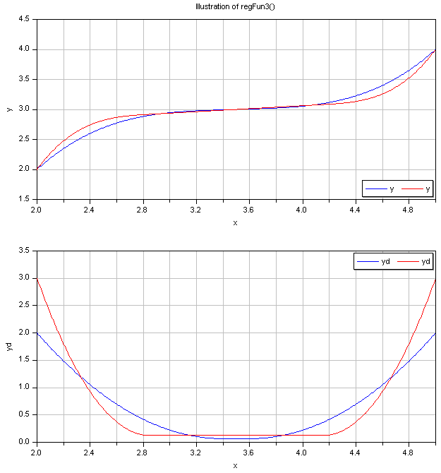
Typical screenshots for two different configurations are shown below. The first one illustrates five different settings of xi and yid:

The second graph shows the continuous derivative of this regularization function:

Literature

Gasparo M. G. and Morandi R. (1991):

Piecewise cubic monotone interpolation with assigned slopes. Computing, Vol. 46, Issue 4, December 1991, pp. 355 - 365.

Interface

function regFun3
  extends Modelica.Icons.Function;
  input Real x "Abscissa value";
  input Real x0 "Lower abscissa value";
  input Real x1 "Upper abscissa value";
  input Real y0 "Ordinate value at lower abscissa value";
  input Real y1 "Ordinate value at upper abscissa value";
  input Real y0d "Derivative at lower abscissa value";
  input Real y1d "Derivative at upper abscissa value";
  output Real y "Ordinate value";
  output Real c "Slope of linear section between two cubic polynomials or dummy linear section slope if single cubic is used";
end regFun3;

Revisions

• May 2008 by Michael Sielemann:
  Designed and implemented.
• February 2011 by Michael Sielemann:
  If the inflection point of the cubic S0 was at +/- infinity, the test criteria of [Gasparo and Morandi, 1991] result in division by zero. This case is handled properly now.
• March 2013 by Michael Sielemann:
  If the arguments prescribed a degenerate case with points (x0,y0) and (x1,y1) on horizontal line, then return value c was undefined. This was corrected. Furthermore, an additional term was included for the computation of y in this case to assist automatic differentiation.