.Modelica.Blocks.Continuous.Filter

Information

This blocks models various types of filters:

low pass, high pass, band pass, and band stop filters

using various filter characteristics:

CriticalDamping, Bessel, Butterworth, Chebyshev Type I filters

By default, a filter block is initialized in steady-state, in order to avoid unwanted oscillations at the beginning. In special cases, it might be useful to select one of the other initialization options under tab "Advanced".

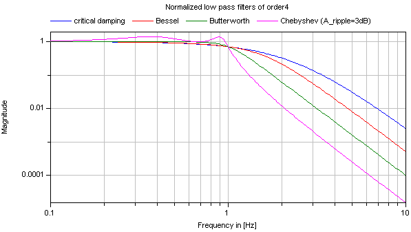
Typical frequency responses for the 4 supported low pass filter types are shown in the next figure:

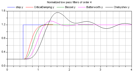
The step responses of the same low pass filters are shown in the next figure, starting from a steady state initial filter with initial input = 0.2:

Obviously, the frequency responses give a somewhat wrong impression of the filter characteristics: Although Butterworth and Chebyshev filters have a significantly steeper magnitude as the CriticalDamping and Bessel filters, the step responses of the latter ones are much better. This means for example, that a CriticalDamping or a Bessel filter should be selected, if a filter is mainly used to make a non-linear inverse model realizable.

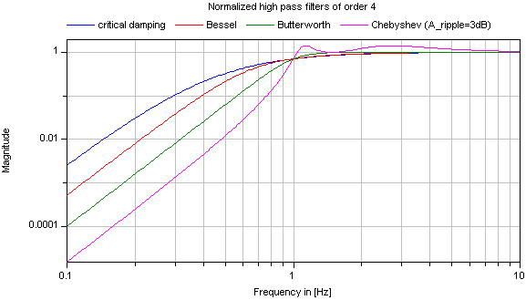
Typical frequency responses for the 4 supported high pass filter types are shown in the next figure:

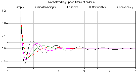
The corresponding step responses of these high pass filters are shown in the next figure:

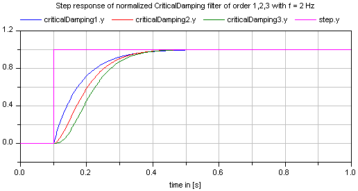
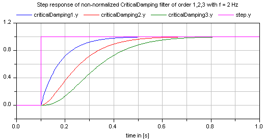
All filters are available in normalized (default) and non-normalized form. In the normalized form, the amplitude of the filter transfer function at the cut-off frequency f_cut is -3 dB (= 10^(-3/20) = 0.70794..). Note, when comparing the filters of this function with other software systems, the setting of "normalized" has to be selected appropriately. For example, the signal processing toolbox of MATLAB provides the filters in non-normalized form and therefore a comparison makes only sense, if normalized = false is set. A normalized filter is usually better suited for applications, since filters of different orders are "comparable", whereas non-normalized filters usually require to adapt the cut-off frequency, when the order of the filter is changed. See a comparison of "normalized" and "non-normalized" filters at hand of CriticalDamping filters of order 1,2,3:

Implementation

The filters are implemented in the following, reliable way:

1. A prototype low pass filter with a cut-off angular frequency of 1 rad/s is constructed from the desired analogFilter and the desired normalization.
2. This prototype low pass filter is transformed to the desired filterType and the desired cut-off frequency f_cut using a transformation on the Laplace variable "s".
3. The resulting first and second order transfer functions are implemented in state space form, using the "eigen value" representation of a transfer function:

   
     // second order block with eigen values: a +/- jb
     der(x1) = a*x1 - b*x2 + (a^2 + b^2)/b*u;
     der(x2) = b*x1 + a*x2;
          y  = x2;
        

   The dc-gain from the input to the output of this block is one and the selected states are in the order of the input (if "u" is in the order of "one", then the states are also in the order of "one"). In the "Advanced" tab, a "nominal" value for the input "u" can be given. If appropriately selected, the states are in the order of "one" and then step-size control is always appropriate.

References

Tietze U., and Schenk C. (2002):

Halbleiter-Schaltungstechnik. Springer Verlag, 12. Auflage, pp. 815-852.

Revisions

Main Author:

Martin Otter, DLR Oberpfaffenhofen.

Acknowledgement

The development of this block was partially funded by BMBF within the ITEA2 EUROSYSLIB project.