Modelica.Mechanics.MultiBody.Joints.Assemblies

Components that aggregate several joints for analytic loop handling

Information

The joints in this package are mainly designed to be used in kinematic loop structures. Every component consists of 3 elementary joints. These joints are combined in such a way that the kinematics of the 3 joints between frame_a and frame_b are computed from the movement of frame_a and frame_b, i.e., there are no constraints between frame_a and frame_b. This requires to solve a non-linear system of equations which is performed analytically (i.e., when a mathematical solution exists, it is computed efficiently and reliably). A detailed description how to use these joints is provided in MultiBody.UsersGuide.Tutorial.LoopStructures.AnalyticLoopHandling.

The assembly joints in this package are named JointXYZ where XYZ are the first letters of the elementary joints used in the component, in particular:

For example, JointUSR is an assembly joint consisting of a universal, a spherical and a revolute joint.

This package contains the following models:

Content

Model	Description
JointUPS	Universal - prismatic - spherical joint aggregation
JointUSR	Universal - spherical - revolute joint aggregation
JointUSP	Universal - spherical - prismatic joint aggregation
JointSSR	Spherical - spherical - revolute joint aggregation with an optional mass point at the rod connecting the two spherical joints
JointSSP	Spherical - spherical - prismatic joint aggregation with an optional mass point at the rod connecting the two spherical joints
JointRRR	Revolute - revolute - revolute joint aggregation for planar loops
JointRRP	Revolute - revolute - prismatic joint aggregation for planar loops

Note, no component of this package has potential states, since the components are designed in such a way that the generalized coordinates of the used elementary joints are computed from the frame_a and frame_b coordinates. Still, it is possible to use the components in a tree structure. In this case states are selected from bodies that are connected to the frame_a or frame_b side of the component. In most cases this gives a less efficient solution, as if elementary joints of package Modelica.Mechanics.MultiBody.Joints would be used directly.

The analytic handling of kinematic loops by using joint aggregations with 6 degrees of freedom as provided in this package, is a new methodology. It is based on a more general method for solving non-linear equations of kinematic loops developed by Woernle and Hiller. An automatic application of this more general method is difficult, and a manual application is only suited for specialists in this field. The method introduced here is a compromise: It can be quite easily applied by an end user, but for a smaller class of kinematic loops. The method of the "characteristic pair of joints" from Woernle and Hiller is described in:

Woernle C.:

Ein systematisches Verfahren zur Aufstellung der geometrischen Schliessbedingungen in kinematischen Schleifen mit Anwendung bei der Rückwärtstransformation für Industrieroboter.
Fortschritt-Berichte VDI, Reihe 18, Nr. 59, Duesseldorf: VDI-Verlag 1988, ISBN 3-18-145918-6.
 

Hiller M., and Woernle C.:

A Systematic Approach for Solving the Inverse Kinematic Problem of Robot Manipulators.
Proceedings 7th World Congress Th. Mach. Mech., Sevilla 1987.

Extends from Modelica.Icons.Package (Icon for standard packages).

Package Content

Name	Description
JointUPS	Universal - prismatic - spherical joint aggregation (no constraints, no potential states)
JointUSR	Universal - spherical - revolute joint aggregation (no constraints, no potential states)
JointUSP	Universal - spherical - prismatic joint aggregation (no constraints, no potential states)
JointSSR	Spherical - spherical - revolute joint aggregation with mass (no constraints, no potential states)
JointSSP	Spherical - spherical - prismatic joint aggregation with mass (no constraints, no potential states)
JointRRR	Planar revolute - revolute - revolute joint aggregation (no constraints, no potential states)
JointRRP	Planar revolute - revolute - prismatic joint aggregation (no constraints, no potential states)

Modelica.Mechanics.MultiBody.Joints.Assemblies.JointUPS

Universal - prismatic - spherical joint aggregation (no constraints, no potential states)

Information

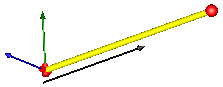
This component consists of a universal joint at frame_a, a spherical joint at frame_b and a prismatic joint along the line connecting the origin of frame_a and the origin of frame_b, see the default animation in the following figure (the axes vectors are not part of the default animation):

This joint aggregation has no mass and no inertia and introduces neither constraints nor potential state variables. It is especially useful to build up more complicated force elements where the mass and/or inertia of the force element shall be taken into account.

The universal joint is defined in the following way:

• The rotation axis of revolute joint 1 is along parameter vector n1_a which is fixed in frame_a.
• The rotation axis of revolute joint 2 is perpendicular to axis 1 and to the line connecting the universal and the spherical joint.

The definition of axis 2 of the universal joint is performed according to the most often occurring case. In a future release, axis 2 might be explicitly definable via a parameter. However, the treatment is much more complicated and the number of operations is considerably higher, if axis 2 is not orthogonal to axis 1 and to the connecting rod.

Note, there is a singularity when axis 1 and the connecting line are parallel to each other. Therefore, if possible n1_a should be selected in such a way that it is perpendicular to nAxis_ia in the initial configuration (i.e., the distance to the singularity is as large as possible).

An additional frame_ia is present. It is fixed on the line connecting the universal and the spherical joint at the origin of frame_a. The placement of frame_ia on this line is implicitly defined by the universal joint (frame_a and frame_ia coincide when the angles of the two revolute joints of the universal joint are zero) and by parameter vector nAxis_ia, an axis vector directed along the line from the origin of frame_a to the spherical joint, resolved in frame_ia.

An additional frame_ib is present. It is fixed in the line connecting the prismatic and the spherical joint at the origin of frame_b. It is always parallel to frame_ia.

Note, this joint aggregation can be used in cases where in reality a rod with spherical joints at each end are present. Such a system has an additional degree of freedom to rotate the rod along its axis. In practice this rotation is usually of no interest and is mathematically removed by replacing one of the spherical joints by a universal joint.

The easiest way to define the parameters of this joint is by moving the MultiBody system in a reference configuration where all frames of all components are parallel to each other (alternatively, at least frame_a, frame_ia and frame_ib of the JointUSP joint should be parallel to each other when defining an instance of this component).

Extends from Interfaces.PartialTwoFramesDoubleSize (Base model for components providing two frame connectors + outer world + assert to guarantee that the component is connected (default icon size is factor 2 larger as usual)).

Parameters

Connectors

Modelica.Mechanics.MultiBody.Joints.Assemblies.JointUSR

Universal - spherical - revolute joint aggregation (no constraints, no potential states)

Information

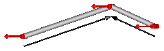
This component consists of a universal joint at frame_a, a revolute joint at frame_b and a spherical joint which is connected via rod1 to the universal and via rod2 to the revolute joint, see the default animation in the following figure (the axes vectors are not part of the default animation):

This joint aggregation has no mass and no inertia and introduces neither constraints nor potential state variables. It should be used in kinematic loops whenever possible since the non-linear system of equations introduced by this joint aggregation is solved analytically (i.e., a solution is always computed, if a unique solution exists).

The universal joint is defined in the following way:

• The rotation axis of revolute joint 1 is along parameter vector n1_a which is fixed in frame_a.
• The rotation axis of revolute joint 2 is perpendicular to axis 1 and to the line connecting the universal and the spherical joint (= rod 1).

The definition of axis 2 of the universal joint is performed according to the most often occurring case. In a future release, axis 2 might be explicitly definable via a parameter. However, the treatment is much more complicated and the number of operations is considerably higher, if axis 2 is not orthogonal to axis 1 and to the connecting rod.

Note, there is a singularity when axis 1 and the connecting rod are parallel to each other. Therefore, if possible n1_a should be selected in such a way that it is perpendicular to rRod1_ia in the initial configuration (i.e., the distance to the singularity is as large as possible).

The rest of this joint aggregation is defined by the following parameters:

• The position of the spherical joint with respect to the universal joint is defined by vector rRod1_ia. This vector is directed from frame_a to the spherical joint and is resolved in frame_ia (it is most simple to select frame_ia such that it is parallel to frame_a in the reference or initial configuration).
• The position of the spherical joint with respect to the revolute joint is defined by vector rRod2_ib. This vector is directed from the inner frame of the revolute joint (frame_ib or revolute.frame_a) to the spherical joint and is resolved in frame_ib (note, that frame_ib and frame_b are parallel to each other).
• The axis of rotation of the revolute joint is defined by axis vector n_b. It is fixed and resolved in frame_b.
• When specifying this joint aggregation with the definitions above, two different configurations are possible. Via parameter phi_guess a guess value for revolute.phi(t0) at the initial time t0 is given. The configuration is selected that is closest to phi_guess (|revolute.phi - phi_guess| is minimal).

An additional frame_ia is present. It is fixed in the rod connecting the universal and the spherical joint at the origin of frame_a. The placement of frame_ia on the rod is implicitly defined by the universal joint (frame_a and frame_ia coincide when the angles of the two revolute joints of the universal joint are zero) and by parameter vector rRod1_ia, the position vector from the origin of frame_a to the spherical joint, resolved in frame_ia.

An additional frame_ib is present. It is fixed in the rod connecting the revolute and the spherical joint at the side of the revolute joint that is connected to this rod (= rod2.frame_a = revolute.frame_a).

An additional frame_im is present. It is fixed in the rod connecting the revolute and the spherical joint at the side of the spherical joint that is connected to this rod (= rod2.frame_b). It is always parallel to frame_ib.

The easiest way to define the parameters of this joint is by moving the MultiBody system in a reference configuration where all frames of all components are parallel to each other (alternatively, at least frame_a and frame_ia of the JointUSR joint should be parallel to each other when defining an instance of this component).

In the public interface of the JointUSR joint, the following (final) parameters are provided:

  parameter Real rod1Length(unit="m")  "Length of rod 1";
  parameter Real eRod1_ia[3] "Unit vector along rod 1, resolved in frame_ia";
  parameter Real e2_ia  [3]  "Unit vector along axis 2, resolved in frame_ia";

This allows a more convenient definition of data which is related to rod 1. For example, if a box shall be connected at frame_ia directing from the origin of frame_a to the middle of rod 1, this might be defined as:

    Modelica.Mechanics.MultiBody.Joints.Assemblies.JointUSP jointUSR(rRod1_ia={1.2, 1, 0.2});
    Modelica.Mechanics.MultiBody.Visualizers.FixedShape     shape(shapeType       = "box",
                                               lengthDirection = jointUSR.eRod1_ia,
                                               widthDirection  = jointUSR.e2_ia,
                                               length          = jointUSR.rod1Length/2,
                                               width           = jointUSR.rod1Length/10);
  equation
    connect(jointUSP.frame_ia, shape.frame_a);

Extends from Interfaces.PartialTwoFramesDoubleSize (Base model for components providing two frame connectors + outer world + assert to guarantee that the component is connected (default icon size is factor 2 larger as usual)).

Parameters

Connectors

Modelica.Mechanics.MultiBody.Joints.Assemblies.JointUSP

Universal - spherical - prismatic joint aggregation (no constraints, no potential states)

Information

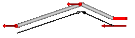
This component consists of a universal joint at frame_a, a prismatic joint at frame_b and a spherical joint which is connected via rod1 to the universal and via rod2 to the prismatic joint, see the default animation in the following figure (the axes vectors are not part of the default animation):

This joint aggregation has no mass and no inertia and introduces neither constraints nor potential state variables. It should be used in kinematic loops whenever possible since the non-linear system of equations introduced by this joint aggregation is solved analytically (i.e., a solution is always computed, if a unique solution exists).

The universal joint is defined in the following way:

• The rotation axis of revolute joint 1 is along parameter vector n1_a which is fixed in frame_a.
• The rotation axis of revolute joint 2 is perpendicular to axis 1 and to the line connecting the universal and the spherical joint (= rod 1).

The definition of axis 2 of the universal joint is performed according to the most often occurring case. In a future release, axis 2 might be explicitly definable via a parameter. However, the treatment is much more complicated and the number of operations is considerably higher, if axis 2 is not orthogonal to axis 1 and to the connecting rod.

Note, there is a singularity when axis 1 and the connecting rod are parallel to each other. Therefore, if possible n1_a should be selected in such a way that it is perpendicular to rRod1_ia in the initial configuration (i.e., the distance to the singularity is as large as possible).

The rest of this joint aggregation is defined by the following parameters:

• The position of the spherical joint with respect to the universal joint is defined by vector rRod1_ia. This vector is directed from frame_a to the spherical joint and is resolved in frame_ia (it is most simple to select frame_ia such that it is parallel to frame_a in the reference or initial configuration).
• The position of the spherical joint with respect to the prismatic joint is defined by vector rRod2_ib. This vector is directed from the inner frame of the prismatic joint (frame_ib or prismatic.frame_a) to the spherical joint and is resolved in frame_ib (note, that frame_ib and frame_b are parallel to each other).
• The axis of translation of the prismatic joint is defined by axis vector n_b. It is fixed and resolved in frame_b.
• The two frames of the prismatic joint, i.e., frame_b and frame_ib, are parallel to each other. The distance between the origins of these two frames along axis n_b is equal to "prismatic.s(t) + s_offset", where "prismatic.s(t)" is a time varying variable and "s_offset" is a fixed, constant offset parameter.
• When specifying this joint aggregation with the definitions above, two different configurations are possible. Via parameter s_guess a guess value for prismatic.s(t0) at the initial time t0 is given. The configuration is selected that is closest to s_guess (|prismatic.s - s_guess| is minimal).

An additional frame_ia is present. It is fixed in the rod connecting the universal and the spherical joint at the origin of frame_a. The placement of frame_ia on the rod is implicitly defined by the universal joint (frame_a and frame_ia coincide when the angles of the two revolute joints of the universal joint are zero) and by parameter vector rRod1_ia, the position vector from the origin of frame_a to the spherical joint, resolved in frame_ia.

An additional frame_ib is present. It is fixed in the rod connecting the prismatic and the spherical joint at the side of the prismatic joint that is connected to this rod (= rod2.frame_a = prismatic.frame_a). It is always parallel to frame_b.

An additional frame_im is present. It is fixed in the rod connecting the prismatic and the spherical joint at the side of the spherical joint that is connected to this rod (= rod2.frame_b). It is always parallel to frame_b.

The easiest way to define the parameters of this joint is by moving the MultiBody system in a reference configuration where all frames of all components are parallel to each other (alternatively, at least frame_a and frame_ia of the JointUSP joint should be parallel to each other when defining an instance of this component).

In the public interface of the JointUSP joint, the following (final) parameters are provided:

  parameter Real rod1Length(unit="m")  "Length of rod 1";
  parameter Real eRod1_ia[3] "Unit vector along rod 1, resolved in frame_ia";
  parameter Real e2_ia  [3]  "Unit vector along axis 2, resolved in frame_ia";

This allows a more convenient definition of data which is related to rod 1. For example, if a box shall be connected at frame_ia directing from the origin of frame_a to the middle of rod 1, this might be defined as:

    Modelica.Mechanics.MultiBody.Joints.Assemblies.JointUSP jointUSP(rRod1_ia={1.2, 1, 0.2});
    Modelica.Mechanics.MultiBody.Visualizers.FixedShape     shape(shapeType       = "box",
                                               lengthDirection = jointUSP.eRod1_ia,
                                               widthDirection  = jointUSP.e2_ia,
                                               length          = jointUSP.rod1Length/2,
                                               width           = jointUSP.rod1Length/10);
  equation
    connect(jointUSP.frame_ia, shape.frame_a);

Extends from Interfaces.PartialTwoFramesDoubleSize (Base model for components providing two frame connectors + outer world + assert to guarantee that the component is connected (default icon size is factor 2 larger as usual)).

Parameters

Connectors

Modelica.Mechanics.MultiBody.Joints.Assemblies.JointSSR

Spherical - spherical - revolute joint aggregation with mass (no constraints, no potential states)

Information

This component consists of a spherical joint 1 at frame_a, a revolute joint at frame_b and a spherical joint 2 which is connected via rod 1 to the spherical joint 1 and via rod 2 to the revolute joint, see the default animation in the following figure (the axes vectors are not part of the default animation):

Besides an optional point mass in the middle of rod 1, this joint aggregation has no mass and no inertia, and introduces neither constraints nor potential state variables. It should be used in kinematic loops whenever possible since the non-linear system of equations introduced by this joint aggregation is solved analytically (i.e., a solution is always computed, if a unique solution exists).

An additional frame_ib is present. It is fixed in rod 2 connecting the revolute and the spherical joint at the side of the revolute joint that is connected to this rod (= rod2.frame_a = revolute.frame_a).

An additional frame_im is present. It is fixed in rod 2 connecting the revolute and the spherical joint at the side of spherical joint 2 that is connected to this rod (= rod2.frame_b). It is always parallel to frame_ib.

The easiest way to define the parameters of this joint is by moving the MultiBody system in a reference configuration where all frames of all components are parallel to each other (alternatively, at least frame_b and frame_ib of the JointSSR joint should be parallel to each other when defining an instance of this component).

Extends from Interfaces.PartialTwoFramesDoubleSize (Base model for components providing two frame connectors + outer world + assert to guarantee that the component is connected (default icon size is factor 2 larger as usual)).

Parameters

Connectors

Modelica.Mechanics.MultiBody.Joints.Assemblies.JointSSP

Spherical - spherical - prismatic joint aggregation with mass (no constraints, no potential states)

Information

This component consists of a spherical joint 1 at frame_a, a prismatic joint at frame_b and a spherical joint 2 which is connected via rod 1 to the spherical joint 1 and via rod 2 to the prismatic joint, see the default animation in the following figure (the axes vectors are not part of the default animation):

Besides an optional point mass in the middle of rod 1, this joint aggregation has no mass and no inertia, and introduces neither constraints nor potential state variables. It should be used in kinematic loops whenever possible since the non-linear system of equations introduced by this joint aggregation is solved analytically (i.e., a solution is always computed, if a unique solution exists).

An additional frame_ib is present. It is fixed in rod 2 connecting the prismatic and the spherical joint at the side of the prismatic joint that is connected to this rod (= rod2.frame_a = prismatic.frame_a).

An additional frame_im is present. It is fixed in rod 2 connecting the prismatic and the spherical joint at the side of spherical joint 2 that is connected to this rod (= rod2.frame_b). It is always parallel to frame_ib.

The easiest way to define the parameters of this joint is by moving the MultiBody system in a reference configuration where all frames of all components are parallel to each other (alternatively, at least frame_b and frame_ib of the JointSSP joint should be parallel to each other when defining an instance of this component).

Extends from Interfaces.PartialTwoFramesDoubleSize (Base model for components providing two frame connectors + outer world + assert to guarantee that the component is connected (default icon size is factor 2 larger as usual)).

Parameters

Connectors

Modelica.Mechanics.MultiBody.Joints.Assemblies.JointRRR

Planar revolute - revolute - revolute joint aggregation (no constraints, no potential states)

Information

This component consists of 3 revolute joints with parallel axes of rotation that are connected together by two rods, see the default animation in the following figure (the axes vectors are not part of the default animation):

This joint aggregation introduces neither constraints nor state variables and should therefore be used in kinematic loops whenever possible to avoid non-linear systems of equations. It is only meaningful to use this component in planar loops. Basically, the position and orientation of the 3 revolute joints as well as of frame_ia, frame_ib, and frame_im are calculated by solving analytically a non-linear equation, given the position and orientation at frame_a and at frame_b.

Connector frame_a is the "left" side of the first revolute joint whereas frame_ia is the "right side of this revolute joint, fixed in rod 1. Connector frame_b is the "right" side of the third revolute joint whereas frame_ib is the "left" side of this revolute joint, fixed in rod 2. Finally, connector frame_im is the connector at the "right" side of the revolute joint in the middle, fixed in rod 2.

The easiest way to define the parameters of this joint is by moving the MultiBody system in a reference configuration where all frames of all components are parallel to each other (alternatively, at least frame_a, frame_ia, frame_im, frame_ib, frame_b of the JointRRR joint should be parallel to each other when defining an instance of this component).

Basically, the JointRRR model consists internally of a universal - spherical - revolute joint aggregation (= JointUSR). In a planar loop this will behave as if 3 revolute joints with parallel axes are connected by rigid rods.

Extends from Interfaces.PartialTwoFramesDoubleSize (Base model for components providing two frame connectors + outer world + assert to guarantee that the component is connected (default icon size is factor 2 larger as usual)).

Parameters

Connectors

Modelica.Mechanics.MultiBody.Joints.Assemblies.JointRRP

Planar revolute - revolute - prismatic joint aggregation (no constraints, no potential states)

Information

This component consists of 2 revolute joints with parallel axes of rotation that and a prismatic joint with a translational axis that is orthogonal to the revolute joint axes, see the default animation in the following figure (the axes vectors are not part of the default animation):

This joint aggregation introduces neither constraints nor state variables and should therefore be used in kinematic loops whenever possible to avoid non-linear systems of equations. It is only meaningful to use this component in planar loops. Basically, the position and orientation of the 3 joints as well as of frame_ia, frame_ib, and frame_im are calculated by solving analytically a non-linear equation, given the position and orientation at frame_a and at frame_b.

Connector frame_a is the "left" side of the first revolute joint whereas frame_ia is the "right side of this revolute joint, fixed in rod 1. Connector frame_b is the "right" side of the prismatic joint whereas frame_ib is the "left" side of this prismatic joint, fixed in rod 2. Finally, connector frame_im is the connector at the "right" side of the revolute joint in the middle, fixed in rod 2. The frames frame_b, frame_ib, frame_im are always parallel to each other.

The easiest way to define the parameters of this joint is by moving the MultiBody system in a reference configuration where all frames of all components are parallel to each other (alternatively, at least frame_a, frame_ia, frame_im, frame_ib, frame_b of the JointRRP joint should be parallel to each other when defining an instance of this component).

Basically, the JointRRP model consists internally of a universal - spherical - prismatic joint aggregation (= JointUSP). In a planar loop this will behave as if 2 revolute joints with parallel axes and 1 prismatic joint are connected by rigid rods.

Extends from Interfaces.PartialTwoFramesDoubleSize (Base model for components providing two frame connectors + outer world + assert to guarantee that the component is connected (default icon size is factor 2 larger as usual)).

Parameters

Connectors