TimeTableGenerate a (possibly discontinuous) signal by linear interpolation in a table |
|
Information
This information is part of the Modelica Standard Library maintained by the Modelica Association.
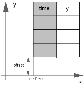
This block generates an output signal by linear interpolation in a table. The time points and function values are stored in a matrix table[i,j], where the first column table[:,1] contains the time points and the second column contains the data to be interpolated. The table interpolation has the following properties:
- The interpolation interval is found by a linear search where the interval used in the last call is used as start interval.
- The time points need to be monotonically increasing.
- Discontinuities are allowed, by providing the same time point twice in the table.
- Values outside of the table range, are computed by extrapolation through the last or first two points of the table.
- If the table has only one row, no interpolation is performed and the function value is just returned independently of the actual time instant.
- Via parameters shiftTime and offset the curve defined by the table can be shifted both in time and in the ordinate value. The time instants stored in the table are therefore relative to shiftTime.
- If time < startTime, no interpolation is performed and the offset is used as ordinate value for the output.
- If the table has more than one row, the first point in time always has to be set to 0, e.g., table=[1,1;2,2] is illegal. If you want to shift the time table in time use the shiftTime parameter instead.
- The table is implemented in a numerically sound way by generating time events at interval boundaries. This generates continuously differentiable values for the integrator.
- Via parameter timeScale the first column of the table array can be scaled, e.g., if the table array is given in hours (instead of seconds) timeScale shall be set to 3600.
Example:
   table = [0, 0;
            1, 0;
            1, 1;
            2, 4;
            3, 9;
            4, 16];
If, e.g., time = 1.0, the output y =  0.0 (before event), 1.0 (after event)
    e.g., time = 1.5, the output y =  2.5,
    e.g., time = 2.0, the output y =  4.0,
    e.g., time = 5.0, the output y = 23.0 (i.e., extrapolation).

Parameters (5)
| offset |
Value: 0 Type: Real Description: Offset of output signal y |
|---|---|
| startTime |
Value: 0 Type: Time (s) Description: Output y = offset for time < startTime |
| table |
Value: fill(0.0, 0, 2) Type: Real[:,2] Description: Table matrix (time = first column; e.g., table=[0, 0; 1, 1; 2, 4]) |
| timeScale |
Value: 1 Type: Time (s) Description: Time scale of first table column |
| shiftTime |
Value: startTime Type: Time (s) Description: Shift time of first table column |
Connectors (1)
| y |
Type: RealOutput Description: Connector of Real output signal |
|---|
Used in Examples (5)
|
Modelica.Blocks.Examples Demonstrates the usage of blocks from Modelica.Blocks.Interaction.Show |
|
|
Modelica.Electrical.PowerConverters.Examples.DCDC.HBridge H bridge DC/DC converter with DC drive |
|
|
Modelica.Magnetic.FluxTubes.Examples.Hysteresis Comparison of the different hysteresis models |
|
|
Modelica.Fluid.Examples.DrumBoiler Complete drum boiler model, including evaporator and supplementary components |
|
|
Modelica.Fluid.Examples.AST_BatchPlant.Test Tank with one time-varying top inlet mass flow rate and a bottom outlet into the ambient |