Modelica.Blocks.Examples.Noise

Library of examples to demonstrate the usage of package Blocks.Noise

Information

This package contains various example models that demonstrates how to utilize the blocks from sublibrary Blocks.Noise.

Extends from Modelica.Icons.ExamplesPackage (Icon for packages containing runnable examples).

Package Content

Name	Description
UniformNoise	Demonstrates the most simple usage of the UniformNoise block
AutomaticSeed	Demonstrates noise with startTime and automatic local seed for UniformNoise
Distributions	Demonstrates noise with different types of distributions
UniformNoiseProperties	Demonstrates the computation of properties for uniformly distributed noise
NormalNoiseProperties	Demonstrates the computation of properties for normally distributed noise
Densities	Demonstrates how to compute distribution densities (= Probability Density Function)
ImpureGenerator	Demonstrates the usage of the impure random number generator
ActuatorWithNoise	Demonstrates how to model measurement noise in an actuator
DrydenContinuousTurbulence	Demonstrates how to model wind turbulence for aircraft with the BandLimitedWhiteNoise block (a simple model of vertical Dryden gust speed at low altitudes < 1000 ft)
Utilities	Library of utility models used in the examples

Modelica.Blocks.Examples.Noise.UniformNoise

Demonstrates the most simple usage of the UniformNoise block

Information

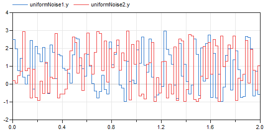
This example demonstrates the most simple usage of the Noise.UniformNoise block:

• globalSeed is the Noise.GlobalSeed block with default options (just dragged from sublibrary Noise).
• uniformNoise1 is an instance of Noise.UniformNoise with samplePeriod = 0.02 s and a Uniform distribution with limits y_min=-1, y_max=3.
• uniformNoise2 is identical to uniformNoise1 with the exception that useAutomaticLocalSeed=false and fixedLocalSeed=10.

At every 0.02 seconds a time event occurs and a uniform random number in the band between -1 ... 3 is drawn. This random number is held constant until the next sample instant. The result of a simulation is shown in the next diagram:

Extends from Modelica.Icons.Example (Icon for runnable examples).

Modelica.Blocks.Examples.Noise.AutomaticSeed

Demonstrates noise with startTime and automatic local seed for UniformNoise

Information

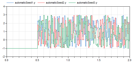
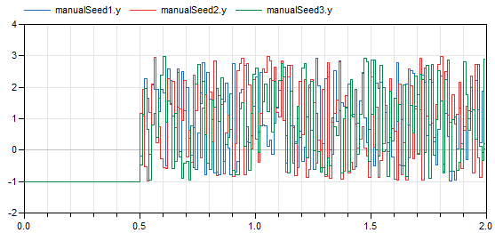
This example demonstrates manual and automatic seed selection of UniformNoise blocks, as well as starting the noise at startTime = 0.5 s with an output value of y = -1 before this time. All noise blocks in this example generate uniform noise in the band y_min=-1 .. y_max=3 with samplePeriod = 0.01 s.

The blocks automaticSeed1, automaticSeed2, automaticSeed3 use the default option to automatically initialize the pseudo random number generators of the respective block. As a result, different noise is generated, see next diagram:

The blocks manualSeed1, manualSeed2, manualSeed3 use manual selection of the local seed (useAutomaticLocalSeed = false). They use a fixedLocalSeed of 1, 2, and 3 respectively. Again, different noise is generated, see next diagram:

Try to set fixedLocalSeed = 1 in block manualSeed2. As a result, the blocks manualSeed1 and manualSeed2 will produce exactly the same noise.

Extends from Modelica.Icons.Example (Icon for runnable examples).

Parameters

Modelica.Blocks.Examples.Noise.Distributions

Demonstrates noise with different types of distributions

Information

This example demonstrates different noise distributions methods that can be selected for a Noise block. Both noise blocks use samplePeriod = 0.02 s, y_min=-1, y_max=3, and have identical fixedLocalSeed. This means that the same random numbers are drawn for the blocks. However, the random numbers are differently transformed according to the selected distributions (uniform and truncated normal distribution), and therefore the blocks have different output values. Simulation results are shown in the next diagram:

As can be seen, uniform noise is distributed evenly between -1 and 3, and truncated normal distribution has more values centered around the mean value 1.

Extends from Modelica.Icons.Example (Icon for runnable examples).

Parameters

Modelica.Blocks.Examples.Noise.UniformNoiseProperties

Demonstrates the computation of properties for uniformly distributed noise

Information

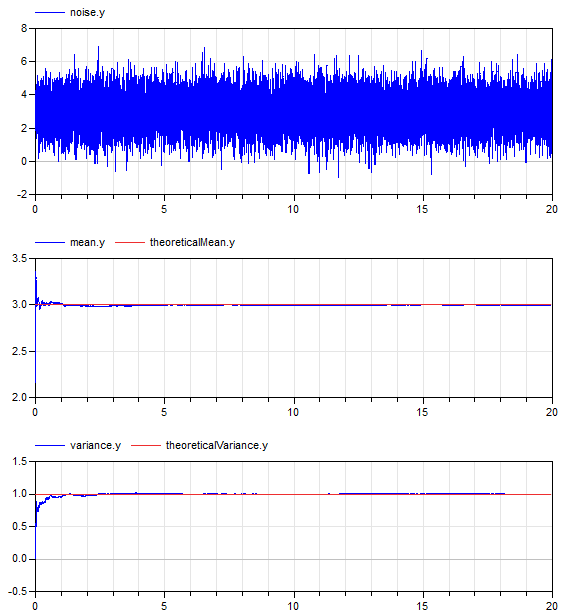
This example demonstrates statistical properties of the Blocks.Noise.UniformNoise block using a uniform random number distribution. Block "noise" defines a band of 0 .. 6 and from the generated noise the mean and the variance is computed with blocks of package Blocks.Math. Simulation results are shown in the next diagram:

The mean value of a uniform noise in the range 0 .. 6 is 3 and its variance is 3 as well. The simulation results above show good agreement (after a short initial phase). This demonstrates that the random number generator and the mapping to a uniform distribution have good statistical properties.

Extends from Modelica.Icons.Example (Icon for runnable examples).

Parameters

Modelica.Blocks.Examples.Noise.NormalNoiseProperties

Demonstrates the computation of properties for normally distributed noise

Information

This example demonstrates statistical properties of the Blocks.Noise.NormalNoise block using a normal random number distribution with mu=3, sigma=1. From the generated noise the mean and the variance is computed with blocks of package Blocks.Math. Simulation results are shown in the next diagram:

The mean value of a normal noise with mu=3 is 3 and the variance of normal noise is sigma^2, so 1. The simulation results above show good agreement (after a short initial phase). This demonstrates that the random number generator and the mapping to a normal distribution have good statistical properties.

Extends from Modelica.Icons.Example (Icon for runnable examples).

Parameters

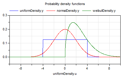
Modelica.Blocks.Examples.Noise.Densities

Demonstrates how to compute distribution densities (= Probability Density Function)

Information

This example demonstrates how to compute the probability density functions (pdfs) of various distributions. In the following diagram simulations results for the uniform, normal, and Weibull distribution are shown. The outputs of the blocks are the pdfs that are plotted over one of the inputs:

Extends from Modelica.Icons.Example (Icon for runnable examples).

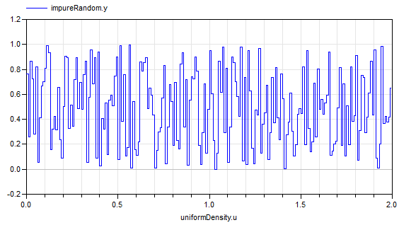
Modelica.Blocks.Examples.Noise.ImpureGenerator

Demonstrates the usage of the impure random number generator

Information

This example demonstrates how to use the impureRandom(..) function to generate random values at event instants. Typically, this approach is only used when implementing an own, specialized block that needs a random number generator. Simulation results are shown in the next figure:

Extends from Modelica.Icons.Example (Icon for runnable examples).

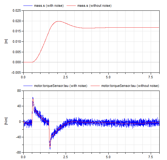
Modelica.Blocks.Examples.Noise.ActuatorWithNoise

Demonstrates how to model measurement noise in an actuator

Information

This example models an actuator with a noisy sensor (which is in the motor component):

The drive train consists of a synchronous motor with a current controller (= motor) and a gear box. The gearbox drives a rod through a linear translation model. Softly attached to the rod is another mass representing the actual actuator (= mass). The actuator is loaded with a constant force.

The whole drive is steered by a rate limited speed step command through a controller model. In the motor the shaft angle is measured and this measurement signal is modelled by adding additive noise to the motor angle.

In the following figure, the position of the actuator and the motor output torque are shown with and without noise. The noise is not very strong, such that it has no visible effect on the position of the actuator. The effect of the noise can be seen in the motor torque.

Note, the noise in all components can be easily switched off by setting parameter enableNoise = false in the globalSeed component.

Extends from Modelica.Icons.Example (Icon for runnable examples).

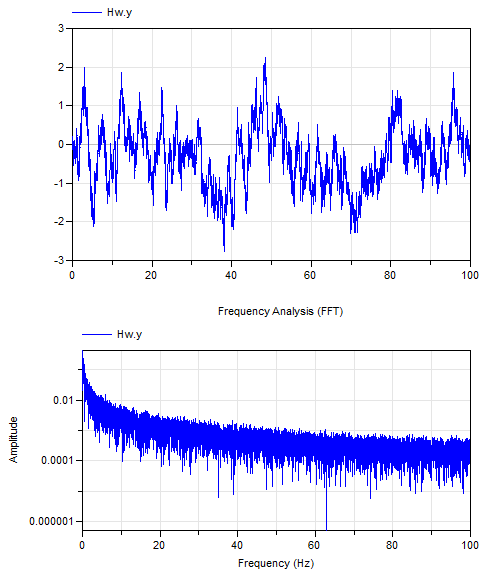
Modelica.Blocks.Examples.Noise.DrydenContinuousTurbulence

Demonstrates how to model wind turbulence for aircraft with the BandLimitedWhiteNoise block (a simple model of vertical Dryden gust speed at low altitudes < 1000 ft)

Information

This example shows how to use the BandLimitedWhiteNoise to feed a Dryden continuous turbulence model. This model is used to describe turbulent wind at low altitudes that varies randomly in space (see also wikipedia).

Turbulence model for vertical gust speed at low altitudes

The turbulence model of the Dryden form is defined by the power spectral density of the vertical turbulent velocity:

The spectrum is parametrized with the following parameters:

• Lw is the turbulence scale.
  In low altitudes, it is equal to the flight altitude.
• sigma is the turbulence intensity.
  In low altitudes, it is equal to 1/10 of the wind speed at 20 ft altitude, which is 30 kts for medium turbulence.
• Omega is the spatial frequency.
  The turbulence model is thus defined in space and the aircraft experiences turbulence as it flies through the defined wind field.
• Omega = s/V will be used to transform the spatial definition into a temporal definition, which can be realized as a state space system.
• V is the airspeed of the aircraft.
  It is approximately 150 kts during the approach (i.e. at low altitudes).

Using spectral factorization and a fixed airspeed V of the aircraft, a concrete forming filter for the vertical turbulence can be found as

,

for which V * (H_w(i Omega/V) * H_w(-i Omega/V) = Phi_w(Omega).

The input to the filter

The input to the filter is white noise with a normal distribution, zero mean, and a power spectral density of 1. That means, for a sampling time of 1s, it is parameterized with mean=0 and variance=1. However, in order to account for the change of noise power due to sampling, the noise must be scaled with sqrt(samplePeriod). This is done automatically in the BandLimitedWhiteNoise block.

Example output

Reference

1. Dryden Wind Turbulence model in US military standard MIL-F-8785.

Extends from Modelica.Icons.Example (Icon for runnable examples).

Parameters