Modelica.Fluid.Dissipation.Utilities.Functions.General

Package with utility functions

Information

Extends from Modelica.Icons.FunctionsPackage (Icon for packages containing functions).

Package Content

Name	Description
CubicInterpolation_Re	Cubic Hermite spline interpolation of the Reynolds number in transition regime of the Moody diagram (inverse formulation)
CubicInterpolation_lambda	Cubic Hermite spline interpolation of the modified friction coefficient in transition regime of the Moody diagram (direct formulation)
LambertW	Closed approximation of Lambert's w function for solving f(x) = x exp(x) for x
LambertWIter	Iterative form of Lambert's w function for solving f(x) = x exp(x) for x
PrandtlNumber	Calculation of Prandtl number
ReynoldsNumber	Calculation of Reynolds number
SmoothPower	Limiting the derivative of function y = if x>=0 then x^pow else -(-x)^pow
SmoothPower_der	The derivative of function SmoothPower
Stepsmoother	Continuous interpolation for x
Stepsmoother_der	Derivative of function Stepsmoother

Modelica.Fluid.Dissipation.Utilities.Functions.General.CubicInterpolation_Re

Cubic Hermite spline interpolation of the Reynolds number in transition regime of the Moody diagram (inverse formulation)

Information

Syntax

Re = CubicInterpolation_Re(0, Re1, Re2, Delta, lambda2);

Description

Function CubicInterpolation_Re(..) approximates the Reynolds number Re in the transition regime between laminar and turbulent flow of the Moody diagram by an inverse formulation of a cubic Hermite spline interpolation. See Modelica.Fluid.UsersGuide.ComponentDefinition.WallFriction (especially Region 2) for a detailed explanation.

Extends from Modelica.Icons.Function (Icon for functions).

Inputs

Outputs

Modelica.Fluid.Dissipation.Utilities.Functions.General.CubicInterpolation_lambda

Cubic Hermite spline interpolation of the modified friction coefficient in transition regime of the Moody diagram (direct formulation)

Information

Syntax

lambda2 = CubicInterpolation_lambda(Re, Re1, Re2, Delta);

Description

Function CubicInterpolation_lambda(..) approximates the modified friction coefficient lambda2=lambda*Re^2 in the transition regime between laminar and turbulent flow of the Moody diagram by a (direct) cubic Hermite spline interpolation. See Modelica.Fluid.UsersGuide.ComponentDefinition.WallFriction (especially Region 2) for a detailed explanation.

Extends from Modelica.Icons.Function (Icon for functions).

Inputs

Outputs

Modelica.Fluid.Dissipation.Utilities.Functions.General.LambertW

Closed approximation of Lambert's w function for solving f(x) = x exp(x) for x

Information

This function calculates an approximation of the inverse for

f(x) = y = x * exp( x )

within ∞ > y > -1/e. The relative deviation of this approximation for Lambert's w function x = W(y) is displayed in the following graph.

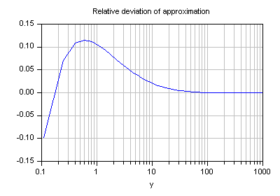
For y > 10 and higher values the relative deviation is smaller 2%.

Extends from Modelica.Icons.Function (Icon for functions).

Inputs

Outputs

Modelica.Fluid.Dissipation.Utilities.Functions.General.LambertWIter

Iterative form of Lambert's w function for solving f(x) = x exp(x) for x

Information

This function calculates an approximation of the inverse for

f(x) = y = x * exp( x )

within ∞ > y > -1/e. Please note, that for negative inputs two solutions exists. The function currently delivers the result x = -1 ... 0 for that particular range.

Extends from Modelica.Icons.Function (Icon for functions).

Inputs

Outputs

Modelica.Fluid.Dissipation.Utilities.Functions.General.PrandtlNumber

Calculation of Prandtl number

Information

Extends from Modelica.Icons.Function (Icon for functions).

Inputs

Outputs

Modelica.Fluid.Dissipation.Utilities.Functions.General.ReynoldsNumber

Calculation of Reynolds number

Information

Extends from Modelica.Icons.Function (Icon for functions).

Inputs

Outputs

Modelica.Fluid.Dissipation.Utilities.Functions.General.SmoothPower

Limiting the derivative of function y = if x>=0 then x^pow else -(-x)^pow

Information

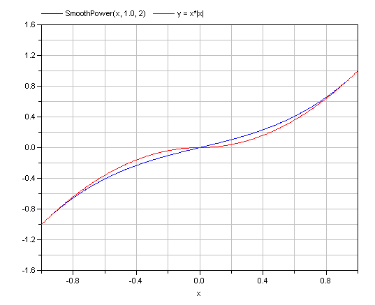
The function is used to limit the derivative of the following function at x=0:

y = if x ≥ 0 then xpow else -(-x)pow;  // pow > 0

by approximating the function in the range -deltax< x < deltax with a third order polynomial that has the same derivative at abs(x)=deltax, as the function above.

Example

In the picture below the input x is increased from -1 to 1. The range of interpolation is defined by the same range. Displayed is the output of the function SmoothPower compared to

y=x*|x|

For |x| > 1 both functions return identical results.

References

ThermoFluid Library

http://sourceforge.net/projects/thermofluid/

Extends from Modelica.Icons.Function (Icon for functions).

Inputs

Outputs

Modelica.Fluid.Dissipation.Utilities.Functions.General.SmoothPower_der

The derivative of function SmoothPower

Information

Extends from Modelica.Icons.Function (Icon for functions).

Inputs

Outputs

Modelica.Fluid.Dissipation.Utilities.Functions.General.Stepsmoother

Continuous interpolation for x

Information

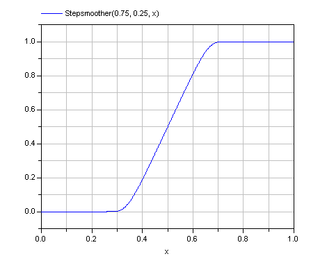
The function is used for continuous fading of variable inputs within a defined range. It allows a differentiable and smooth transition between function outputs, e.g., laminar and turbulent pressure drop or correlations for certain ranges.

Function

The tanh-function is used, since it provides an existing derivative and the derivative is zero at the borders [nofunc, func] of the interpolation domain (smooth derivative for transitions).

In order to work correctly, the internal interpolation range in terms of the external arbitrary input x needs to be scaled such that:

f(func)   = 0.5 π
f(nofunc) = -0.5 π

Example

In the picture below the input x is increased from 0 to 1. The range of interpolation is defined by:

• func = 0.75
• nofunc = 0.25

References

Wischhusen, St.

Simulation von Kältemaschinen-Prozessen mit MODELICA / DYMOLA. Diploma thesis, Hamburg University of Technology, Institute of Thermofluiddynamics, 2000.

Extends from Modelica.Icons.Function (Icon for functions).

Inputs

Outputs

Modelica.Fluid.Dissipation.Utilities.Functions.General.Stepsmoother_der

Derivative of function Stepsmoother

Information

Extends from Modelica.Icons.Function (Icon for functions).

Inputs

Outputs