Modelica.Fluid.Dissipation.Utilities.SharedDocumentation.PressureLoss.Orifice

Extends from Modelica.Icons.Information (Icon for general information packages).

Package Content

Name	Description
dp_suddenChange
dp_thickEdgedOverall

Modelica.Fluid.Dissipation.Utilities.SharedDocumentation.PressureLoss.Orifice.dp_suddenChange

Restriction

This function shall be used within the restricted limits according to the referenced literature.

• Smooth surface
• Turbulent flow regime
• Reynolds number for sudden expansion Re > 3.3e3 [Idelchik 2006, p. 208, diag. 4-1]
• Reynolds number for sudden contraction Re > 1e4 [Idelchik 2006, p. 216-217, diag. 4-9]

Geometry

Calculation

The local pressure loss dp is generally determined by:

dp = 0.5 * zeta_LOC * rho * |v_1|*v_1

with

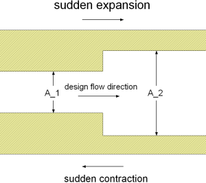
The local resistance coefficient zeta_LOC of a sudden expansion can be calculated for different ratios of cross sectional areas by:

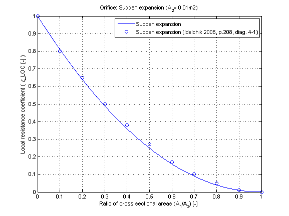
zeta_LOC = (1 - A_1/A_2)^2  [Idelchik 2006, p. 208, diag. 4-1]

and for sudden contraction:

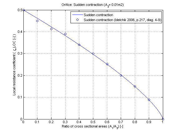
zeta_LOC = 0.5*(1 - A_1/A_2)^0.75  [Idelchik 2006, p. 216-217, diag. 4-9]

with

Verification

The local resistance coefficient zeta_LOC of a sudden expansion in dependence of the cross sectional area ratio A_1/A_2 is shown in the figure below.

The local resistance coefficient zeta_LOC of a sudden contraction in dependence of the cross sectional area ratio A_1/A_2 is shown in the figure below.

References

Elmqvist, H., M.Otter and S.E. Cellier:

Inline integration: A new mixed symbolic / numeric approach for solving differential-algebraic equation systems.. In Proceedings of European Simulation MultiConference, Prague, 1995.

Idelchik,I.E.:

Handbook of hydraulic resistance. Jaico Publishing House, Mumbai, 3rd edition, 2006.

Extends from Modelica.Icons.Information (Icon for general information packages).

Modelica.Fluid.Dissipation.Utilities.SharedDocumentation.PressureLoss.Orifice.dp_thickEdgedOverall

Restriction

This function shall be used within the restricted limits according to the referenced literature.

• Reynolds number (for vena contraction) Re > 1e3 [Idelchik 2006, p. 222, diag. 4-15]
• Relative length of vena contraction (L/d_hyd_0) > 0.015 [Idelchik 2006, p. 222, diag. 4-15]
• Darcy friction factor lambda_FRI = 0.02 [Idelchik 2006, p. 222, sec. 4-15]

Geometry

Calculation

The pressure loss dp for a thick edged orifice is determined by:

dp = zeta_TOT * (rho/2) * (velocity_1)^2

with

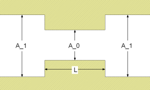
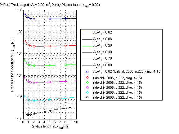
The pressure loss coefficient zeta_TOT of a thick edged orifice can be calculated for different cross sectional areas A_0 and relative length of orifice l_bar = L/d_hyd_0 by:

zeta_TOT = (0.5*(1 - A_0/A_1)^0.75 + tau*(1 - A_0/A_1)^1.375 + (1 - A_0/A_1)^2 + lambda_FRI*l_bar)*(A_1/A_0)^2 [Idelchik 2006, p. 222, diag. 4-15]

with

The geometry factor tau is determined by [Idelchik 2006, p. 219, diag. 4-12]:

tau = (2.4 - l_bar)*10^(-phi)
phi = 0.25 + 0.535*l_bar^8 / (0.05 + l_bar^8) .

Verification

The pressure loss coefficient zeta_TOT of a thick edged orifice in dependence of a relative length (l_bar = L /d_hyd) with different ratios of cross sectional areas A_0/A_1 is shown in the figure below.

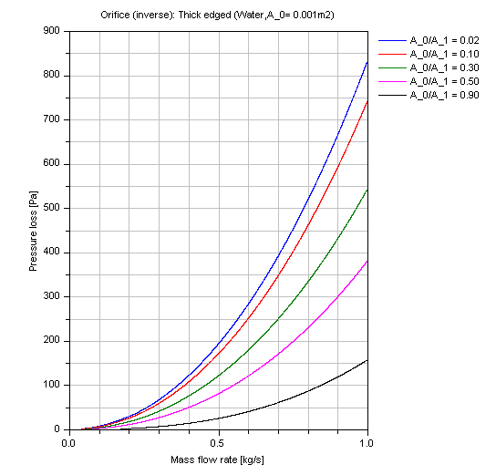
Incompressible case [Pressure loss = f(m_flow)]:

The pressure loss DP of an thick edged orifice in dependence of the mass flow rate m_flow of water for different ratios A_0/A_1 (where A_0 = 0.001 m^2) is shown in the figure below.

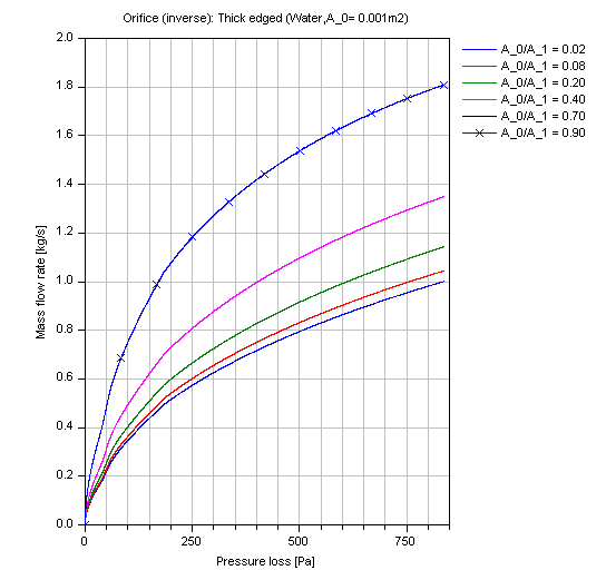
And for the compressible case [Mass flow rate = f(dp)]:

References

Elmqvist,H., M.Otter and S.E. Cellier:

Inline integration: A new mixed symbolic / numeric approach for solving differential-algebraic equation systems.. In Proceedings of European Simulation MultiConference, Prague, 1995.

Idelchik,I.E.:

Handbook of hydraulic resistance. Jaico Publishing House,Mumbai, 3rd edition, 2006.

Extends from Modelica.Icons.Information (Icon for general information packages).