.Modelica.Fluid.Dissipation.Utilities.SharedDocumentation.PressureLoss.General.dp_nominalPressureLossLawDensity

Information

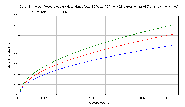
Calculation of a generic pressure loss in dependence of nominal fluid variables (e.g., nominal density) via interpolation from an operation point. This generic function considers the pressure loss law via a nominal pressure loss (dp_nom), a pressure loss coefficient (zeta_TOT) and a pressure loss law exponent (exp) as well as the influence of density on pressure loss.

Calculation

The geometry parameters of energy devices necessary for the pressure loss calculations are often not exactly known. Therefore the modelling of the detailed pressure loss calculation have to be simplified. This function uses nominal variables (e.g., nominal pressure loss) at a known operation point of the energy device to interpolate the actual pressure loss according to a pressure loss law (exponent).

In the following the pressure loss dp is generally determined from a known operation point via a law of similarity:

   dp/dp_nom = (zeta_TOT/zeta_TOT_nom)*(rho/rho_nom)*(v/v_nom)^exp

with

The fraction of mean flow velocities (v/v_nom) can be calculated through its corresponding mass flow rates , densities and cross sectional areas:

   v/v_nom = (m_flow/m_flow_nom)*(A_cross_nom/A_cross)*(rho_nom/rho)

or through its corresponding volume flow rates , densities and cross sectional areas:

    v/v_nom = (V_flow/V_flow_nom)*(A_cross_nom/A_cross).

with

Here the compressible case [Mass flow rate = f(dp)] determines the unknown mass flow rate out of a given pressure loss:

   m_flow = m_flow_nom*(A_cross/A_cross_nom)*(rho_nom/rho)^(exp_density/exp)*[(dp/dp_nom)*(zeta_TOT_nom/zeta_TOT)]^(1/exp);

where the exponent for the fraction of densities is determined w.r.t. the chosen nominal mass flow rate or nominal volume flow rate to:

  exp_density = if NominalMassFlowRate == Modelica.Fluid.Dissipation.Utilities.Types.MassOrVolumeFlowRate.MassFlowRate then 1-exp else 1

with

To avoid numerical difficulties this pressure loss function is linear smoothed for small pressure losses, with

   dp ≤ 0.01*dp_nom

Note that the input and output arguments for functions throughout this library always use mass flow rates. Here you can choose NominalMassFlowRate == Modelica.Fluid.Dissipation.Utilities.Types.MassOrVolumeFlowRate.MassFlowRate for using a nominal mass flow rate or NominalMassFlowRate == Modelica.Fluid.Dissipation.Utilities.Types.MassOrVolumeFlowRate.VolumeFlowRate for using a nominal volume flow rate. The output argument will always be a mass flow rate for further use as flow model in a thermo-hydraulic framework.

Note that the pressure loss coefficients (zeta_TOT,zeta_TOT_nom) refer to its mean flow velocities (v,v_nom) in the pressure loss law to obtain its corresponding pressure loss.

Verification

Compressible case [Mass flow rate = f(dp)]:

The generic mass flow rate M_FLOW in dependence of the pressure loss dp is shown for a turbulent pressure loss regime (exp == 2) in the figure below.

Note that the verification for dp_nominalPressureLossLawDensity is also valid for this inverse calculation due to using the same functions.

References

Elmqvist, H., M.Otter and S.E. Cellier:

Inline integration: A new mixed symbolic / numeric approach for solving differential-algebraic equation systems.. In Proceedings of European Simulation MultiConference, Praque, 1995.

Wischhusen, S.:

Dynamische Simulation zur wirtschaftlichen Bewertung von komplexen Energiesystemen.. PhD thesis, Technische Universität Hamburg-Harburg, 2005.